How has the number of persons seeking protection in Germany changed over time?
A stacked area chart using {ggplot2}
Overview
In Germany, as of 31 December 204, according to the Central Register of Foreigners, more than 14 million people of the 83.6 Million residents are foreigners.
It is important to note, that about 3.3 Million arrived to the country seeking protection. This figure is about 78% larger than the reported in 2020, and 343% more than 10 years ago.
An effective tool to analyze these data is through stacked area charts that allow to visualize the evolution of the variable of interest, persons seeking protection in this case, disaggregating it by categories. In this post, I will create a stacked area chart of this information using {ggplot2} in R.
About the data
Data are produced by the Central Register of Foreigners and are presented by Statistisches Bundesamt (Destatis) in their website in Table Persons seeking protection, by protection status, 2007 to 2024. I downloaded this information and saved it in an Excel file named persons-seeking-protection-germany.xlsx.
Set-up
First, I load the packages to be used:
Loading data
I downloaded Table Persons seeking protection, by protection status, 2007 to 2024 and saved it in an Excel file named persons-seeking-protection-germany.xlsx.
seeking_protection <- read_excel("persons-seeking-protection-germany.xlsx")The table looks like this:
seeking_protection |>
  kbl(
    caption = "Persons seeking protection, by protection status, 2007 to 2024"
    ) |>
kable_paper("hover", full_width = F)| Reference date | Population | Foreign population | Persons seeking protection | unsettled | recognised | temporary | permanent | refused |
|---|---|---|---|---|---|---|---|---|
| 31 December 2007 | 82217837 | 6744880 | 457430 | 20145 | 301995 | 164350 | 137650 | 135290 |
| 31 December 2008 | 82002356 | 6727620 | 456050 | 18930 | 330365 | 150795 | 179570 | 106755 |
| 31 December 2009 | 81802257 | 6694775 | 477595 | 24620 | 361775 | 158735 | 203040 | 91195 |
| 31 December 2010 | 81751602 | 6753620 | 503470 | 35835 | 382325 | 168205 | 214115 | 85310 |
| 31 December 2011 | 80327900 | 6930895 | 505925 | 47130 | 373875 | 151045 | 222825 | 84920 |
| 31 December 2012 | 80523746 | 7213710 | 549825 | 65920 | 399050 | 165610 | 233440 | 84860 |
| 31 December 2013 | 80767463 | 7633630 | 613925 | 110335 | 410570 | 174110 | 236460 | 93020 |
| 31 December 2014 | 81197537 | 8152970 | 746320 | 177900 | 460140 | 208460 | 251675 | 108280 |
| 31 December 2015 | 82175684 | 9107895 | 1036235 | 349810 | 547935 | 285805 | 262130 | 138495 |
| 31 December 2016 | 82521653 | 10039080 | 1597570 | 574945 | 867500 | 599235 | 268265 | 155120 |
| 31 December 2017 | 82792351 | 10623940 | 1680700 | 348640 | 1154365 | 888355 | 266010 | 177700 |
| 31 December 2018 | 83019214 | 10915455 | 1781750 | 306095 | 1283225 | 1017760 | 265465 | 192430 |
| 31 December 2019 | 83166711 | 11228300 | 1839115 | 266470 | 1360070 | 1090475 | 269590 | 212575 |
| 31 December 2020 | 83155031 | 11432460 | 1856785 | 215960 | 1397685 | 1116970 | 280715 | 243140 |
| 31 December 2021 | 83237124 | 11817790 | 1936350 | 238945 | 1451375 | 1133545 | 317835 | 246030 |
| 31 December 2022 | 83118501 | 13383910 | 3078650 | 570060 | 2253875 | 1916630 | 337245 | 254710 |
| 31 December 2023 | 83456045 | 13895865 | 3173135 | 454795 | 2528935 | 2188665 | 340275 | 189405 |
| 31 December 2024 | 83577140 | 14061640 | 3304705 | 427415 | 2706320 | 2377115 | 329205 | 170970 |
Designing the stacked area chart
Before plotting, I reshape the data and rename some of their columns for easiness of working with them in the {ggplot2} context.
seeking_protection <- seeking_protection |>
  # I use year() to extract the information of the year
  mutate(year = year(dmy(`Reference date`))) |>
  # Only the subset of variables to use
  select(year, unsettled, temporary, permanent, refused) |>
  # Lengthening the data
  pivot_longer(!year,
              names_to = "status",
              values_to = "persons")
First, I set a theme for the chart and the font to “Josefin Sans” using the showtext package. More options can be found at https://fonts.google.com/.
font_add_google("Josefin Sans", "Josefin Sans")

showtext_auto()

theme_stacked_chart <- function() {
  theme_minimal(
    base_family = "Josefin Sans"
  ) +
    # Custom settings
    theme(

      # Title settings
      plot.title.position = "plot",
      plot.title = element_textbox(
        color = "#800000",
        face = "bold",
        size = 20,
        margin = margin(5, 0, 15, 0), # top, right, bottom, left
        hjust = 0,
        halign = 0      ),

      plot.subtitle = element_textbox(
      color = "#767676",
      #face = "bold",
      size = 18,
      margin = margin(5, 0, 35, 0),
      hjust = 0,
      halign = 0
      ),

      # Axis settings
      axis.line = element_line(
        size = 1.1,
        colour = "#800000"
        ),

      axis.title.y = element_text(
        color = "#800000",
        face = "bold",
        size = 16
      ),
      axis.text.y = element_text(
        color = "#800000",
        face = "bold",
        size = 13
      ),
      axis.title.x = element_blank(),
      axis.text.x = element_text(
        color = "#800000",
        face = "bold",
        size = 13
      ),

      # Legend settings
      legend.position.inside = c(0.15, 0.80),
      legend.title = element_text(
        color = "#800000",
        face = "bold",
        size = 14
      ),
      legend.text = element_text(
        color = "#800000",
        size = 13
      ),

      # Caption settings
      plot.caption = element_text(
        color = "#800000",
        face = "italic",
        size = 14,
        hjust = 0,
        margin = margin(20, 0, 5, 0), # top, right, bottom, left
        ),

      plot.background = element_rect(
        color = "#D6D6CE",
        fill = "#D6D6CE"
      ),
      plot.margin = margin(40, 40, 40, 40) # top, right, bottom, left
    )
}
The plot is created with the following code:
seeking_protection <- seeking_protection |>
  mutate(status = str_to_title(status))

ggplot(seeking_protection,
  aes(
      x = year,
      y = persons,
      fill = status,
      color = status
      )
    ) +
  geom_area() +
  guides(fill = guide_legend(title = "Protection status",
                             position = "inside"),
         color = guide_legend(title = "Protection status",
                             position = "inside")
                             ) +
  scale_fill_manual(
    values = c("Unsettled"= "#767676",
               "Temporary"= "#CC8214",
               "Refused" = "#8A9045",
               "Permanent" = "#155F83"
               )
  ) +
  scale_color_manual(
    values = c("Unsettled"= "#767676",
               "Temporary"= "#CC8214",
               "Refused" = "#8A9045",
               "Permanent" = "#155F83"
               )
  ) +
  scale_y_continuous(
    labels = label_number(
      scale = 1e-6
      )
    ) +
  scale_x_continuous(
    expand = c(0, 0),
    limits = c(2006.5, 2024.5),
    breaks = seq(2007, 2024, by = 1)
  ) +
  labs(
    title = "Persons seeking protection in Germany by status | 2007-2024",
    y = "Number of persons \n(in Millions)",
    caption = "Source: Central Register of Foreigners. \nDesign: Juan Torres Munguía."
    ) +
theme_stacked_chart() showtext_opts(dpi = 320)
ggsave(
"stacked-area-germany-seeking-protection.png",
dpi = 320,
width = 12,
height = 9,
units = "in"
)
showtext_auto(FALSE) # Turn off the showtext functionality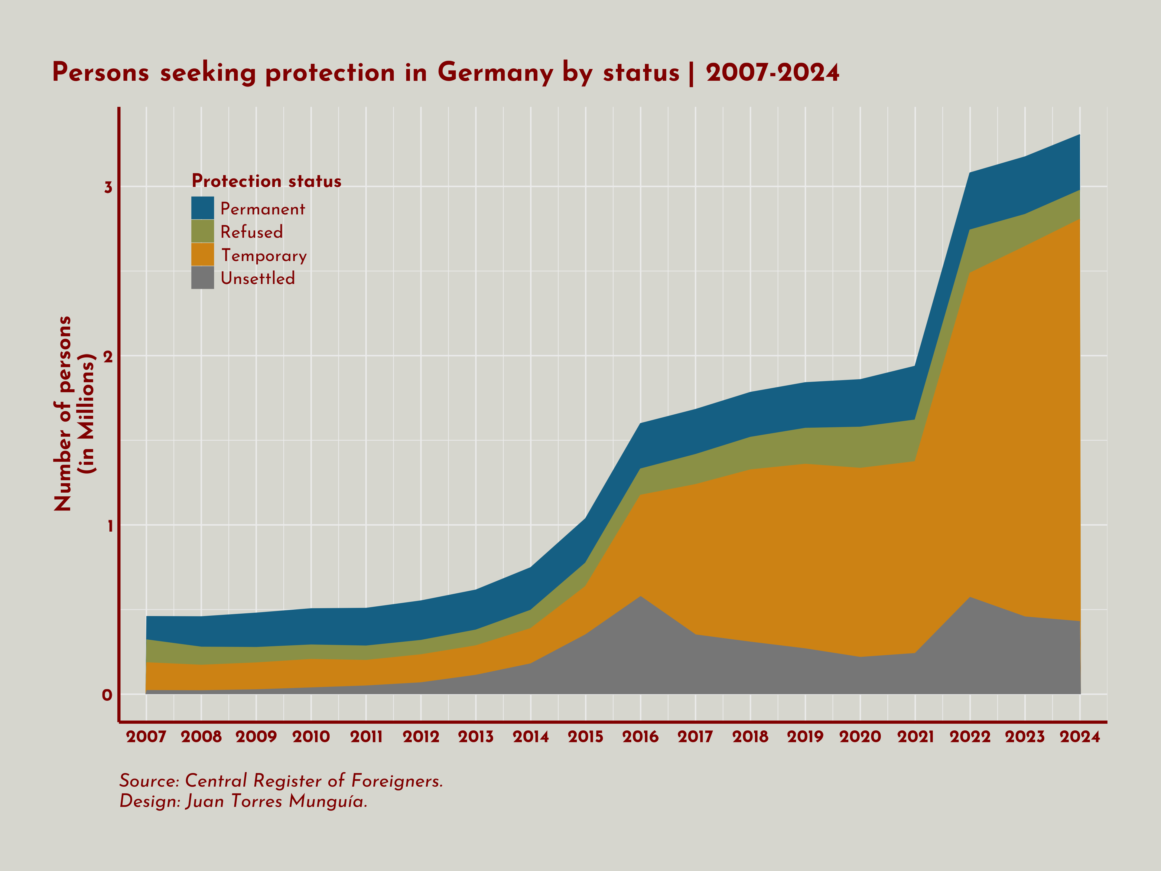
Citation
@online{torres munguía2025,
  author = {Torres Munguía, Juan Armando},
  title = {How Has the Number of Persons Seeking Protection in {Germany}
    Changed over Time?},
  date = {2025-08-01},
  url = {https://juan-torresmunguia.netlify.app/blog/posts/germany-persons-seeking-protection-stacked-area-chart},
  langid = {en}
}